xhtml | css

MMBGX is a package for analysing whole-transcript Affymetrix arrays at the Ensembl gene or Ensembl transcript (isoform) level, taking into account the multi-mapping structure between probes and the features they target. The package relies on the annmap Bioconductor package to create the "structure directories" containing the mapping information linking probes to features. The oligo Bioconductor package is needed to map probes to oligonucleotide sequences. Please cite Turro et al. 2010 if you use this software in your work. Note that, in contrast to the description in the paper, MMBGX now runs separately on each array and condition-specific expression estimates can be generated afterwards as described below. Additionally, MMBGX now uses annmap mappings rather than Affymetrix mappings for Gene ST arrays as well as Exon ST arrays.
makeStructDir command in R. E.g. suppose you have installed the human Ensembl 70 database and named it "hs70" in the databases.txt file (as explained in the annmap cookbook PDF), then you could create the structure directory for analysing HuEx-1_0-st-v2 arrays at the transcript level as follows: makeStructDir(annmapDB="hs70", cdfName="HuEx-1_0-st-v2", geneLevel=FALSE). Alternatively, if you are having trouble getting the MySQL database to work or simply wish to save some time, you can download the Ensembl 64 gene and transcript level structure directories for HuEx-1_0-st-v2 and HuGene-1_0-st-v1 arrays here. Ensembl 70 directories for HuEx-1_0-st-v2 (transcript and gene level), MoGene-1_0-st-v1 (gene level) and MoEx-1_0-st-v1 (transcript and gene level) are available here. Unzip the file and place the structDirs directory inside the mmbgx R library directory (echo `R RHOME`/library/mmbgx). If you would like to be sent structure directories for other array types, species or versions of Ensembl, please contact the corresponding author.cond1 and cond2 respectively.
library(mmbgx)
setwd("cond1")
d <- read.celfiles(dir())
mmbgx(d, geneLevel=FALSE, outputDir="transcriptRuns")
mmbgx(d, geneLevel=TRUE, outputDir="geneRuns")
setwd("../cond2")
d <- read.celfiles(dir())
mmbgx(d, geneLevel=FALSE, outputDir="transcriptRuns")
mmbgx(d, geneLevel=TRUE, outputDir="geneRuns")
setwd("..")
This will analyse each Exon array CEL file in directory cond1 at the transcript and gene level. The output of the transcript-level analysis will go in directories named run.1, run.2, run.3, etc. inside cond1/transcriptRuns/. The output of the gene-level analysis will end up in cond1/geneRuns/ The same will happen in directory cond2. Type ?mmbgx for documentation. Note that each array may be analysed simultaneously. If you have many arrays and a computing cluster, we recommend using the standalone binary.
combineRuns.mmbgx(c(dir("cond1/transcriptRuns", full.names=TRUE), dir("cond2/transcriptRuns", full.names=TRUE)), sampleSets=c(3,3), outputDir="combinedTranscriptRun")
combineRuns.mmbgx(c(dir("cond1/geneRuns", full.names=TRUE), dir("cond2/geneRuns", full.names=TRUE)), sampleSets=c(3,3), outputDir="combinedGeneRun")
This will loess-normalise all the arrays and average the posterior distributions of the expression parameter "mu" within conditions.
resG <- readSingle.mmbgx("combinedGeneRun")
resT <- readSingle.mmbgx("combinedTranscriptRun")
You may then access several data structures. E.g.:
resT$PSids: a vector of probeset IDs (Affy gene IDs for Gene arrays; Ensembl transcript IDs (if geneLevel=FALSE) or gene IDs (if geneLevel=TRUE) for Exon arrays). In the case of Exon arrays, you may occasionally see IDs formed from multiple IDs separated by the '+' character (E.g. ENST00000009120+ENST00000234610 or ENSG00000123584+ENSG00000166008. That is because these transcripts or genes cannot be distinguished using the available probes on the array. You should treat the expression for these probesets as the aggregate expression of all the component transcripts/genes.resT$muave: the log expression estimate of each probeset (rows) under each condition (columns)resT$mu[[n]]: 1024 posterior samples of the log expression parameter for each probeset (rows) under condition nresT$geneIDs (for transcript-level Exon array analysis only): list of Ensembl gene IDsresT$geneTranscripts (only available for Exon array data): mappings from Ensembl genes to Ensembl transcript IDsIt is useful to plot a histogram of the probability of up-regulation of each transcript or gene (cf. Hein et al. 2006, Figure 4). The peaks near 0 and 1 in the example below represent differentially expressed genes/transcripts while the hump around 0.5 represents the non-differentially expressed set. If the spline fit (the black line) is inadequate, try setting a lower value for the df argument. Type ?analysis.mmbgx for documentation.
plotDEHistogram(resT)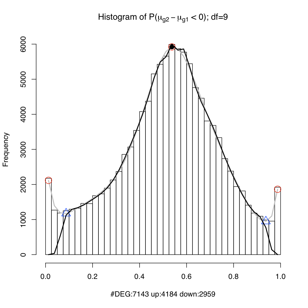
The genes/transcripts may be ranked by differential expression.
> ra <- rankByDE(resT, absolute=TRUE)
> head(ra)
                                Position DiffExpression
ENST00000382159                    33819       424.4531
ENST00000381340+ENST00000451599    33387       412.2417
ENST00000261637                     3963       384.4219
ENST00000371079                    26935       373.2364
ENST00000334258                    15571       365.8463
ENST00000358117                    21671       365.2377
> plotDEDensity(resT, "ENST00000382159")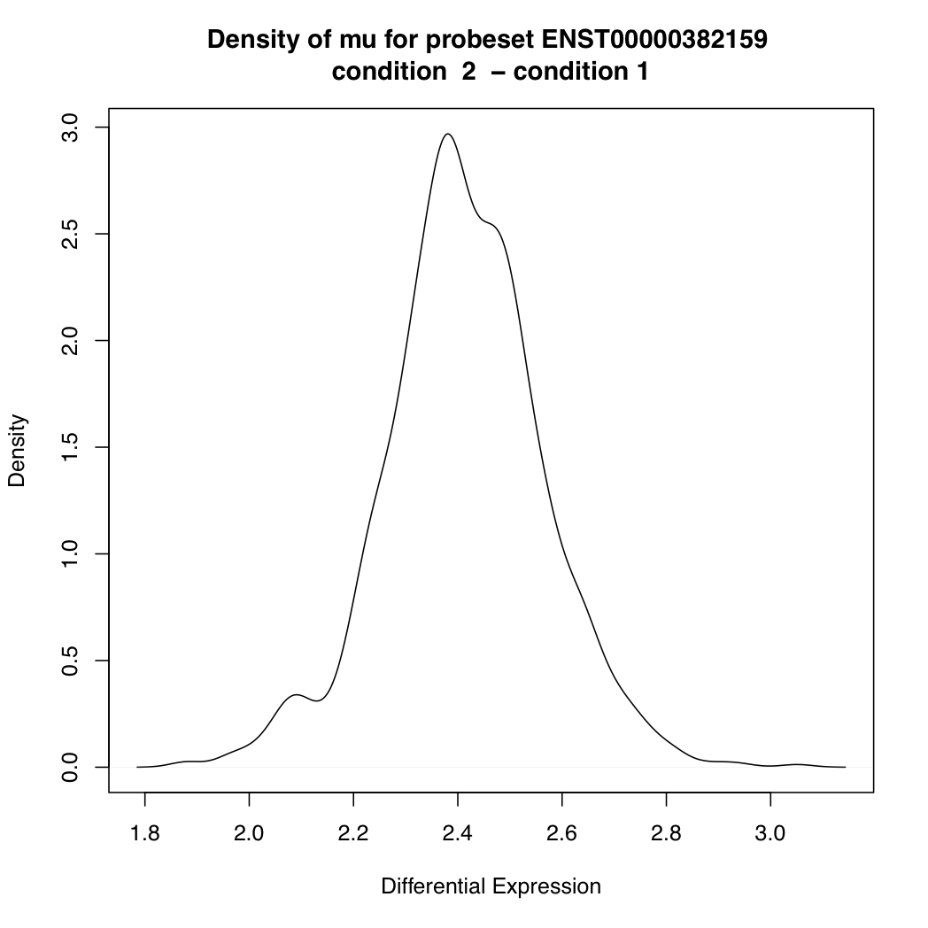
> tail(ra)
Position DiffExpression
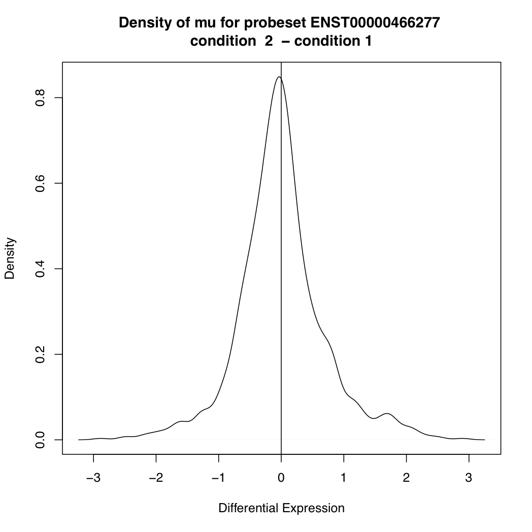
ENST00000466277 88301 0.0004721673
ENST00000360019 22569 0.0002682017
ENST00000474642 95186 0.0002639391
ENST00000461757 84570 0.0001762428
ENST00000395730 38539 0.0001606146
ENST00000328642 14258 0.0001176768
> plotDEDensity(resT, 88301)
The main goal of differential splicing analysis is to identify transcripts whose expression change between conditions is significantly different from the overall expression change of its gene:
ds <- differentialSplicing(resG, resT)
ds is a data frame with four columns:
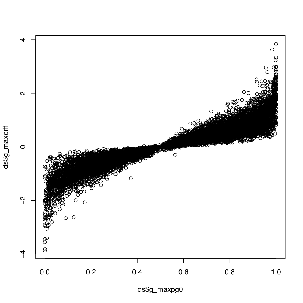
g_index: the gene index in resT$geneIDsg_maxpg0: the maximum value within a gene for the probability that a transcript's differential expression is greater than that of its geneg_maxdiff: the log fold change for the transcript with the maximum value abovet_index: the index of the transcript with the most extreme value aboveg_transconsidered: the number of transcripts considered when calculating the above valuesg_maxpg0 near 0 or 1 and a relatively high abs(g_maxdiff). This plot may be useful:
plot(ds$g_maxpg0, ds$g_maxdiff)
> head(ds[(ds$g_maxpg0 > 0.95 | ds$g_maxpg0 < 0.05) & abs(ds$g_maxdiff) > 2.5,])
40       66 1.00000000  2.976158  111067                 8
104     168 0.02929688 -2.646944   76121                 2
128     218 0.00000000 -3.558733   57454                 7
192     304 0.00000000 -2.710747   28648                14
280     449 1.00000000  2.710265  106233                 8
645    1003 0.00781250 -3.058512  109931                18

> resT$geneIDs[ds$g_index[2]]
[1] "ENSG00000000457"

>  resT$PSids[ds$t_index[2]]
[1] "ENST00000367772"
You can plot the posterior densities of expression parameter "mu" for the various transcripts under each condition:
plotTranscriptDensities(resT, ds$g_index[2])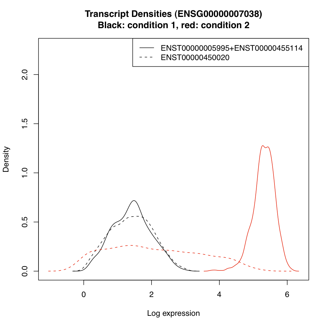
The MMBGX software is computationally intensive so you should try to run it on a powerful computer with lots of CPU cores. If you are analysing many arrays, you might prefer to run the standalone binary on a cluster to speed things up.
To run MMBGX as a standalone binary, you must first compile it. Then, from R, run the mmbgx function with inputDirs set to a character vector of length equal to the number of arrays in the AffyBatch object and standalone=TRUE (each element of inputDirs is a temporary directory of your choice, one per array). You can then run the standalone binary once per array, passing path/to/inputdir/infile.txt as a single argument each time. E.g.
From the command line (just do this once):
tar -xzf mmbgx_0.99.27.tar.gz
cd mmbgx/src/
make -f Makefile.standalone
Before you run make above, you might want to check that -march is set appropriately for your machine in the Makefile.standalone file.
I have found that ICC-compiled binaries are about twice as fast as GCC-compiled ones. If you use 64-bit linux, I recommend you try the ICC-compiled statically-linked binary mmbgx-icc in the src/ directory.
Then in R, prepare the input directories:
library(mmbgx)
setwd("cond1")
d <- read.celfiles(dir())
# create input directories transcriptInput.1, transcriptInput.2, ..., geneInput.1, geneInput.2...
mmbgx(d, geneLevel=FALSE, inputDirs=paste("transcriptInput", c(1:length(d)), sep="."), standalone=TRUE)
mmbgx(d, geneLevel=TRUE, inputDirs=paste("geneInput", c(1:length(d)), sep="."), standalone=TRUE)
setwd("../cond2")
d <- read.celfiles(dir())
mmbgx(d, geneLevel=FALSE, inputDirs=paste("transcriptInput", c(1:length(d)), sep="."), standalone=TRUE)
mmbgx(d, geneLevel=TRUE, inputDirs=paste("geneInput", c(1:length(d)), sep="."), standalone=TRUE)
From the command line run MMBGX:
cd cond1; mkdir transcriptRuns; mkdir geneRuns
cd transcriptRuns
for i in `ls .. | grep transcriptInput.`; do
  ../../mmbgx/src/mmbgx $i/infile.txt
done
cd ../geneRuns
for i in `ls .. | grep geneInput.`; do
  ../../mmbgx/src/mmbgx $i/infile.txt
done
cd ../../cond2; mkdir transcriptRuns; mkdir geneRuns
# etc
libgomp.so.1: shared object cannot be dlopen()ed after library(mmbgx), restart R as follows: LD_PRELOAD=libgomp.so.1 R.
cd /usr/bin
sudo rm gcc cc g++
sudo ln -s gcc-4.2 gcc
sudo ln -s gcc-4.2 cc
sudo ln -s g++-4.2 g++
cd /Library/Frameworks/R.framework/Versions/Current/Resources/etc/i386/
sudo sed -i .bak 's/-isysroot\ \/Developer\/SDKs\/MacOSX10\.4u\.sdk//g' Makeconf
cd /Library/Frameworks/R.framework/Versions/Current/Resources/etc/i386/
sudo cp Makeconf.bak Makeconf