xhtml | css

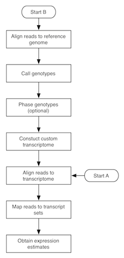
The flowchart to the right depicts the MMSEQ pipeline for obtaining expression estimates from RNA-seq data. There are two routes, with starting points labelled A and B. Route A is quite fast and straightforward to run and uses pre-existing transcript sequences for alignment. Route B requires more time, as it involves the creation of custom transcript sequences based on the data. The two routes are described below. Basic knowledge of how to work in a unix-based environment is required. Route A may be run through the R-based ArrayExpressHTS pipeline. Please cite Turro et al. 2011 (Genome Biology) if you use MMSEQ in your work.
bam2hits updates: print nice ASCII insert size histogram to check it's roughly normal; -i option now uses expected_isize and sd_of_isizes (instead of deviation_thres); unless adjusted lengths are provided or calculated with mseq (options -c and -u), transcript lengths are adjusted using the insert size distribution - the prior fragment distribution given the transcript is assumed to be uniform up to the transcript length within the main support of the insert size distribution; proper repetitive transcript filter applied before simplified isize deviation filter; deal gracefully with truncated hits files)hitstools utility; fixed default regex to work with new (>v64) Ensembl fasta entry naming convention; more information in *.mmseq tables; output gzipped MCMC traces; improved readmmseq.R script)*.mmseq files now contain all the transcripts or genes, regardless of whether they have counts; improved R script to read in the output (readmmseq.R); fixed potential integer overflow if gibbs_iter set too high; default gibbs_iter doubled to 2^14, though there can be a noticeable reduction in autocorrelation up to 2^17 iterations)yum install mmseq). Many thanks to Adam Huffman.bam2hits)haploref.rb works properly with custom regular expressions - same behaviour as testregexp.rb and bam2hits; fixed bug in identical transcript/gene amalgamation code. Prior to 0.9.10, incorrect values outputted in *.amalgamated.mmseq and *.gene.mmseq files if one of the transcripts had zero hits and no values outputted in *.gene.mmseq for genes with log Gibbs mean < 0)MMSEQ consists of two main binaries (bam2hits and mmseq) and several supporting utilities (binaries and Ruby, Perl and bash scripts). Make sure the directories containing the Bowtie, SAMtools and MMSEQ binaries and scripts are in your PATH, otherwise some of the commands in this manual will not work (see Note 8).
extract_transcripts program included in the MMSEQ package, but note that it only works with Ensembl-like GTF files. Usage: extract_transcripts genome_fasta ensembl_gtf_file > transcript_fasta.-m "(.*)" 1 1 in bam2hits (see below), which ignores the gene level.bowtie-build. It is advisable to use a lower-than-default value for --offrate (such as 2 or 3) as long as the resulting index fits in memory. E.g. if you're using the ready-made filtered file for Human, try:
gunzip Homo_sapiens.GRCh37.64.ref_transcripts.fa.gz
bowtie-build --offrate 3 Homo_sapiens.GRCh37.64.ref_transcripts.fa Homo_sapiens.GRCh37.64.ref_transcripts
trim_galore --phred64 -q 15 -a AGATCGGAAGAGCACACGTCTGAACTCCAGTCACTAACAAGATCTCGTATGCCGTCTTCTGCTTG \
  -a2 AGATCGGAAGAGCGTCGTGTAGGGAAAGAGTGTAGATCTCGGTGGTCGCCGTATCATT -s 3 -e 0.05 \
--length 36 --trim1 --gzip --paired file_1.fq.gz file_2.fq.gz-a --best --strata -S (you absolutely must remember to specify -a to ensure you get multi-mapping alignments). Suppress alignments for reads that map to a huge number of transcripts with the -m option (e.g. -m 100). Other flags/options may be needed depending on your data (e.g. -I and -X for the minimum and maximum insert size and/or --norc if you are using a forward-stranded protocol). If your reference FASTA file doesn't use the vertebrate Ensembl naming convention, then you must specify --fullref. If you are using barcoding and the read names of your second mates end with /3 or /4, you need to change your FASTQ files so that they end with /2 instead because bowtie only trims read names ending with /1 or /2 (awk 'FNR % 4==1 { sub(/\/[34]$/, "/2") } { print }' secondreads.fq > secondreads-new.fq should do the trick). If you have multiple FASTQ files from the same library, feed them all together to Bowtie in one go (separate the FASTQ file names with commas). If you are getting many "Exhausted best-first chunk memory" warnings, try increasing --chunkmbs to 128 or 256. If the read names contain any spaces, make sure the substring up to the first space in each read is unique, as Bowtie strips anything after a space in a read name. The output BAM file must be sorted by read name. With paired-end data, only pairs where both reads have been aligned are used so you can use the samtools 0xC filtering flag to reduce the size of your output. E.g. to align the paired files 3125_7_1.fastq and 3125_7_2.fastq (from the Montgomery et al. HapMap data):
bowtie -a --best --strata -S -m 100 -X 400 --chunkmbs 256 -p 8 Homo_sapiens.GRCh37.64.ref_transcripts \
  -1 3125_7_1.fastq -2 3125_7_2.fastq | samtools view -F 0xC -bS - | samtools sort -n - 3125_7.namesorted
bam2hits. Basic usage: bam2hits transcript_fasta namesorted_bam > hits_file (run bam2hits with no arguments for full usage instructions and see Notes 3, 4, 5 and 6 for additional guidance). E.g.:
bam2hits Homo_sapiens.GRCh37.64.ref_transcripts.fa 3125_7.namesorted.bam > 3125_7.hits
hitstools utility.
mmseq program. Basic usage: mmseq hits_file output_base (run mmseq without arguments for full usage instructions). E.g.:
mmseq 3125_7.hits 3125_7
output_base.mmseq contains a table with columns:
output_base.identical.mmseq: as above but aggregated over transcripts sharing the same sequence (these estimates are usually far more precise than the corresponding individual estimates in the transcript-level table). Note that log_mu_em and proportion summaries are not available for aggregates.output_base.gene.mmseq: as above but aggregated over genes and the effective_length is an average of isoform effective lengths weighted by their expressionoutput_base.*.trace_gibbs.gz, output_base.M and output_base.k). These will be useful for downstream analysis in future, but they can be ignored for now.MMSEQ consists of three binaries (bam2hits, mmseq and extract_transcripts) and several Ruby, R, Perl and bash scripts. Make sure the directories containing the Bowtie, TopHat, SAMtools and MMSEQ binaries and scripts are in your PATH, otherwise some of the commands in this manual will not work. Also, add the path to polyHap2.jar to the CLASSPATH, otherwise the Java commands in this manual will not work (see Note 8).
fastagrep.sh script included with the MMSEQ package (see Note 2). Alternatively, use the ready-made filtered transcript FASTA file for Human (Ensembl v64, gzipped).fastagrep.sh script included with the MMSEQ package (see Note 2). Alternatively, use the ready-made filtered genome FASTA file for Human (Ensembl v64, gzipped).
gene → mRNA → exon structure in the third column (as in the Ensembl-derived files).
bowtie-build. E.g. bowtie-build -f Homo_sapiens.GRCh37.64.dna.toplevel.ref.fa Homo_sapiens.GRCh37.64.dna.toplevel.ref. Alternatively, download ready-made Bowtie indexes for Human (Ensembl v64 (GRCh37/hg19), gzipped).--no-novel-juncs --min-isoform-fraction 0.0 --min-anchor-length 3. The output directory should be specified with the -o option. This example is based on the Montgomery et al. HapMap dataset:
tophat -G Homo_sapiens.GRCh37.64.ref.gff --no-novel-juncs --min-isoform-fraction 0.0 --min-anchor-length 3 \
       -r 192 -p 8 -o 3125_7.tophat Homo_sapiens.GRCh37.64.dna.toplevel.ref 3125_7_1.fastq 3125_7_2.fastq
SBAMS=( `find . -wholename "*.tophat/accepted_hits.bam"` )
samtools mpileup -ugf Homo_sapiens.GRCh37.64.dna.toplevel.ref.fa ${SBAMS[@]} | bcftools view -bvcg - > var.raw.bcf
bcftools view var.raw.bcf | vcfutils.pl varFilter > var.flt.vcf
java dataFormat.ImportSNPs Homo_sapiens.GRCh37.64.ref.gff var.flt.vcf ph2temp
phase.sh script in the temporary directory. E.g.:
./ph2temp/phase.shphase.sh may safely be run simultaneously if you have access to many CPUs.phase.sh script with the -r option to assign the alleles to the two haplotypes without phasing (REF alleles are assigned to the _A haplotype and ALT alleles to the _B haplotype). This option may be used even when the number of samples is as low as 1.
java dataFormat.ConvertABtoATGC Homo_sapiens.GRCh37.64.ref.gff ph2temp ph2outputhaploref.rb script. Usage: haploref.rb transcript_fasta gff_file pos_file hap_file > hapiso_fasta. E.g. for sample 3125_7:
haploref.rb ../Homo_sapiens.GRCh37.64.ref_transcripts.fa ../Homo_sapiens.GRCh37.64.ref.gff SNPinfo 3125_7.hap > 3125_7.fa
The mmdiff binary allows you to perform model comparison using the MMSEQ output. You can run mmdiff as follows:
mmdiff [OPTIONS...] matrices_file mmseq_file1 mmseq_file2... > out.mmdiffSet the prior probability that the second model is true with -p FLOAT. Use the option -useprops to model summaries of the posterior isoform proportions rather than the expression levels from MMSEQ. Run the binary without arguments for more options.
The matrices files determines which models you wish to compare. You must define four matrices: M is a model-independent covariate matrix, C maps observations to classes for each model, P0(collapsed) is a collapsed matrix (i.e. distinct rows) defining statistical model 0 and P1(collapsed) is a collapsed matrix defining statistical model 1. If a model has no classes (i.e. just an intercept term) use 1 for the P matrix. E.g. for differential expression between two groups of 4 samples without extraneous variables the following matrices file would be appropriate:
# M; no. of rows = no. of observations
0
0
0
0
0
0
0
0
# C; no. of rows = no. of observations and no. of columns = 2 (one for each model)
0 0
0 0
0 0
0 0
0 1
0 1
0 1
0 1
# P0(collapsed); no. of rows = no. of classes for model 0
1
# P1(collapsed); no. of rows = no. of classes for model 1
.5
-.5
For a three-way differential expression analysis with three, three and two observations per group respectively, the following matrices file would be appropriate:
# M; no. of rows = no. of observations
0
0
0
0
0
0
0
0
# C; no. of rows = no. of observations and no. of columns = 2 (one for each model)
0 0
0 0
0 0
0 1
0 1
0 1
0 2
0 2
# P0(collapsed); no. of rows = no. of classes for model 0
1
# P1(collapsed); no. of rows = no. of classes for model 1
1 0 0
0 1 0
0 0 1
In order to assess whether the log fold change between group A and group B is different to the log fold change between group C and group D, assuming there are two observations per group, the following matrices file would be appropriate:
# M; no. of rows = no. of observations
0
0
0
0
0
0
0
0
# C; no. of rows = no. of observations and no. of columns = 2 (one for each model)
0 0
0 0
0 1
0 1
1 2
1 2
1 3
1 3
# P0(collapsed); no. of rows = no. of classes for model 0
.5
-.5
# P1(collapsed); no. of rows = no. of classes for model 1
.5 .5
.5 -.5
-.5 .5
-.5 -.5
If you require advice on setting up the matrices file for your particular study design, do not hesitate to contact the corresponding author.
Description of the output:
The MMSEQ expression estimates are in FPKM units (fragments per kilobase of transcript per million mapped reads or read pairs), which makes different samples broadly comparable. You may read in the output from multiple samples using the readmmseq.R R script included in the MMSEQ package (requires R ≥ 2.9). The readmmseq function takes three arguments:
mmseq_files: vector of *.mmseq output files to read insample_names: vector of strings containing the sample namesnormalize: logical scalar specifying whether to normalise the log expression values and log count equivalents for each sample by their median deviation from the mean (like DESeq).The function returns a list with the following elements:
log_mu_gibbs: the expression estimatesmcse: the standard errorscounts: the count equivalentsunique_hits: the number of unique hits per featureeffective_length: the effective lengths, which differ across samplestrue_length: the actual lengths of the transcript sequencesTo test for differential expression with edgeR or DESeq, the count equivalents need to be used. E.g., to test for DE between two groups of two samples, you might run the following code in R from the directory containing the mmseq output files:
source("/path/to/readmmseq.R")
library(edgeR)
library(DESeq) # version >=1.5

ms = readmmseq()
tab = ms$counts[apply(ms$counts,1,function(x) any(round(x)>0)),] # only keep features with counts

# edgeR
d = DGEList(counts = tab, group = c("group1", "group1", "group2","group2"))
d = estimateCommonDisp(d)
de.edgeR = exactTest(d)

# DESeq
cds = newCountDataSet(round(tab), c("group1", "group1", "group2", "group2") )
sizeFactors(cds) = rep(1, dim(cds)[2])
cds = estimateDispersions(cds)
de.DESeq = nbinomTest(cds,"group1", "group2")
The mmcollapse binary takes the outputs from mmseq and collapses sets of transcripts based on posterior correlation estimates. The overall precision of the expression estimates for a collapsed set is usually much greater than for the individual component transcripts, which typically share important structural features (many shared exons, etc). Usage:
mmcollapse basename1 basename2...
Here, basename is the name of the mmseq output files without the suffixes (.mmseq, .identical.mmseq, .gene.mmseq). The output is a set of new MMSEQ files with suffix .collapsed.mmseq.
The MMSEQ package comes with statically-linked binaries for 64-bit Mac OS X and GNU/Linux and should work out of the box on most systems. On Fedora 14/15 and EPEL 5/6 systems, you can install the package simply by running yum install mmseq. If you prefer to compile the binaries yourself, you will need the following dependencies:
port install boostbrew install boost; ln -s /usr/local/lib/libboost_regex-mt.a /usr/local/lib/libboost_regex.a; ln -s /usr/local/lib/libboost_iostreams-mt.a /usr/local/lib/libboost_iostreams.aapt-get install libboost-all-devyum install boost (or, on older systems, yum install boost141)brew install samtools; export CPLUS_INCLUDE_PATH=$CPLUS_INCLUDE_PATH:/usr/local/include/bamTo compile the binaries in the MMSEQ package with GCC, simply run make. Due to a bug in the default version of GCC that comes with XCode for Mac OS X, you need to use a more recent version of GCC. If the Boost, GSL or SAMtools libraries aren't found by the compiler, add the path(s) containing the header files and libraries respectively to the LIBRARY_PATH and CPLUS_INCLUDE_PATH environment variables. E.g. to add the path to SAMtools (which should contain sam.h and libbam.a, among other files):
export CPLUS_INCLUDE_PATH=/home/bob/seq/samtools-0.1.17:$CPLUS_INCLUDE_PATH
export LIBRARY_PATH=/home/bob/seq/samtools-0.1.17:$LIBRARY_PATH
If you still can't compile and you can't or don't want to use the pre-packaged binaries, please contact the corresponding author on the paper.
You must also make sure you have a Ruby interpreter to run the Ruby scripts. It comes bundled with Mac OS X and often with GNU/Linux. It is easy to install on the latter with a package manager:
apt-get install ruby-fullyum install rubyIf you wish to correct the transcript lengths for non-uniformity effects using the Poisson regression method of Li et al., you must install the R package mseq.
fastagrep.sh is similar to unix grep except it works on multi-line sequence entries in a FASTA file. E.g., to remove alternative haplotype/supercontig entries from the Ensembl DNA, cDNA and ncRNA FASTA files and combine the filtered cDNA and ncRNA files:
fastagrep.sh -v 'supercontig|GRCh37:Y:1:10000|GRCh37:[^1-9XMY]' Homo_sapiens.GRCh37.64.dna.toplevel.fa > Homo_sapiens.GRCh37.64.dna.toplevel.ref.fa
fastagrep.sh -v 'supercontig|GRCh37:[^1-9XMY]' Homo_sapiens.GRCh37.64.cdna.all.fa > Homo_sapiens.GRCh37.64.cdna.ref.fa
fastagrep.sh -v 'supercontig|GRCh37:[^1-9XMY]' Homo_sapiens.GRCh37.64.ncrna.fa > Homo_sapiens.GRCh37.64.ncrna.ref.fa
cp Homo_sapiens.GRCh37.64.cdna.ref.fa Homo_sapiens.GRCh37.64.ref_transcripts.fa
cat Homo_sapiens.GRCh37.64.ncrna.ref.fa >> Homo_sapiens.GRCh37.64.ref_transcripts.fa
(note how this gets rid of the pesky 'GRCh37:Y:1:10000' entry in Ensembl human DNA FASTA files, which only contains Ns and breaks samtools indexing)
It is possible to use reference transcript FASTA files with entries that are formatted differently than the cDNA and ncRNA files provided by Ensembl. To do this, tell bam2hits how to access the transcript IDs and the gene IDs in the reference entries using the -m tg_regexp t_ind g_ind option. tg_regexp specifies a regular expression that matches FASTA entries (excluding the >) where pairs of brackets are used to capture transcript and gene IDs. t_ind and g_ind are indexes for which pair of brackets capture the transcript and gene IDs respectively. E.g. for the human Ensembl file, entries look like this:
>ENST00000416067 cdna:known chromosome:GRCh37:21:9907194:9968585:-1 gene:ENSG00000227328so (assuming you ran bowtie with --fullref) you can tell bam2hits how to extract the transcript and gene IDs like this:
bam2hits -m "(E\S+).*gene:(E\S+).*" 1 2 Homo_sapiens.GRCh37.64.ref_transcripts.fa 3125_7.sam > 3125_7.hitsIf you are unsure what regular expression to use, try out by trial and error using the testregexp.rb script. Usage: testregexp.rb -m tg_regexp t_ind g_ind transcript_fasta. If you run bam2hits with the -m option, double-check the IDs in the header and main lines of the output hits file before feeding it to mmseq (use the hitstools utility to inspect binary hits files or convert them to text format).
For paired-end data, bam2hits obtains the mode of the insert size distribution from the first 2M proper pairs with unambiguous insert sizes, smoothing the histogram in windows of 3, and sets it to the expected insert size, while the standard deviation is set to 1/1.96 times the distance between the mode and the top 2.5% insert sizes. For single-end data, the mean and standard deviation are set to 180 and 25 respectively. These values can be overridden with the -i expected_isize sd_of_isizes option.
The normal approximation is used to give transcripts their effective lengths. If you would like to adjust the lengths differently, specify -u alt_lengths in bam2hits, where alt_lengths is the name of a previously produced file containing the transcript IDs and the adjusted lengths in a two column layout.
Additionally, for paired-end reads, an insert size deviation filter removes alignments with insert sizes beyond 1.96 sd of the mean if alternative alignments exist with insert sizes within 1.96 sd of the mean. The filter can be disabled with -k.
You may correct the transcript lengths for non-uniformity effects with Poisson regression method of Li et al. by specifying the -c alt_lengths option when running bam2hits, where alt_lengths is the name of an output file in which to save the adjusted lengths for future use. This is quite a time-consuming task, so if you have multiple runs with similar non-uniformity biases, you may choose to use the adjusted lengths calculated from one run when processing a subsequent run. This can be achieved by specifying -u alt_lengths in bam2hits, where alt_lengths is the name of a previously produced file containing the transcript IDs and the adjusted lengths in a two column layout. Currently the Li et al. correction and the insert size distribution correction (above) are mutually exclusive, but a combined correction is in the works.
If you are not interested in haplo-isoform estimation and have constructed a new transcript reference with arbitrary-phase haplo-isoform sequences solely to reduce allelic mapping biases, then the alignments to the "_A" and "_B" haplo-isoforms should be merged. This can be done by specifying the -b flag when running bam2hits.
Once you have downloaded a GTF file from Ensembl, run the filterGTF.rb and ensembl_gtf_to_gff.pl scripts to remove GTF entries which are not in the transcript FASTA and convert to GFF. E.g. for human:
filterGTF.rb Homo_sapiens.GRCh37.64.ref_transcripts.fa Homo_sapiens.GRCh37.64.gtf > Homo_sapiens.GRCh37.64.ref.gtf
ensembl_gtf_to_gff.pl Homo_sapiens.GRCh37.64.ref.gtf > Homo_sapiens.GRCh37.64.ref.gff
# rename bundled Mac OS X binaries
unzip mmseq_1.0.2.zip && cd mmseq_1.0.2
mv bam2hits-1.0.2-Darwin-x86_64 bam2hits
mv mmseq-1.0.2-Darwin-x86_64 mmseq
mv mmdiff-1.0.2-Darwin-x86_64 mmmdiff
#...

# set paths for mmseq and samtools binaries and scripts
export PATH=$PATH:/home/bob/mmseq_1.0.2:/home/bob/samtools:/home/bob/samtools/misc

# set java path for polyHap2
export CLASSPATH=$CLASSPATH:/home/bob/polyHap2_20110607/polyHap2.jar
mmseq with the OMP_NUM_THREADS environment variable.